
Why Synthetic Atmospheric Look-Alikes Outperform Unpaired Real Smoke Footage in Early-Warning Training
Enlarging a training set with thousands of additional real-world wildfire smoke images fails to establish better precision on deployed optical camera networks. When a convolutional detector views an incipient plume against a complex ridgeline, its primary failure mode rarely stems from an inability to recognize dense smoke. False dispatches occur because the model has never mapped the decision boundary between early pyrolysis and localized atmospheric interference occupying the exact same terrain geometry.
Field observation of wildland camera networks demonstrates how background entanglement skews model weights. If an archive contains real ignitions captured primarily during dry afternoon conditions on south-facing slopes, and benign fog events captured at dawn in shaded valleys, a classifier trained on that raw footage simply learns to associate ridge profiles and solar elevation with fire. Controlled ablation checks change that dynamic entirely. By testing three distinct regimes in parallel—real imagery alone, real imagery augmented with synthetic smoke, and real imagery paired with both synthetic smoke and matched hard-negative atmospheric look-alikes—engineering teams can isolate whether the network recognizes aerosol plume physics or merely memorizes lighting correlates.
Suppressing false alarms for emergency response requires generating paired synthetic smoke and hard-negative atmospheric confounders across identical background plates. For every pristine horizon frame extracted from a hilltop tower, the generative pipeline renders an active combustion plume alongside matched negative examples of orographic lifting fog, agricultural dust plumes, industrial steam, and solar lens flare. Preserving the exact camera pose, terrain crop, and illumination vector across both the positive and negative synthetic injections forces the feature extractor to evaluate translucency gradients and upward buoyancy rather than ridge topography.
The Four-Stage Operational Pipeline
Executing this hard-negative priority protocol across wildland camera networks requires four sequential engineering phases:
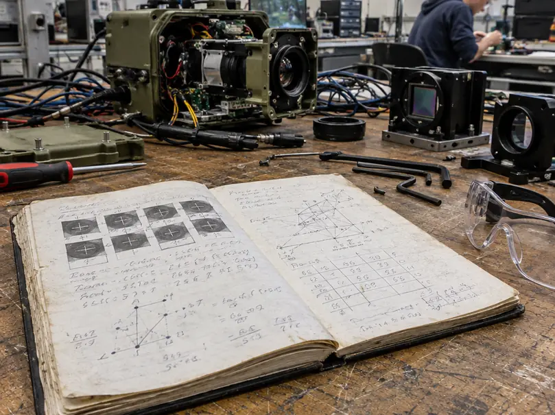
- Baseline Background Curation: Isolating uncontaminated horizon plates from repeatable pan-tilt-zoom (PTZ) tower presets, locking solar geometry and meteorological telemetry into a strict relational schema while separating terrestrial captures from satellite monitoring datasets.
- Physically Constrained Fluid-to-GAN Rendering: Driving an Eulerian fluid solver to generate time-resolved volumetric density and velocity fields, then passing those optical depth maps through a conditional adversarial translator to synthesize photorealistic billow textures without altering plume geometry.
- Radiometric Domain Adaptation: Degrading the pristine generative composites through a forward sensor model that replicates distance-dependent atmospheric transmission, CMOS dark current, image signal processor (ISP) sharpening, and H.264/H.265 compression macroblocking.
- Curriculum Injection and Shadow Calibration: Balancing real and synthetic pairs inside the object detection training loop, incorporating multi-frame temporal verification, and validating dispatch precision during a 14-to-28-day shadow evaluation on live camera streams before enabling automated alerts.
Curating Terrestrially Paired Background Substrates and Confounder Taxonomies
A paired synthetic curriculum is only as reliable as the alignment of its underlying terrain substrates. Hilltop PTZ forestry cameras experience mechanical backlash, thermal mast expansion, and wind buffeting. Before extracting empty horizon plates, group all raw observations by their repeatable PTZ preset identifiers and run an automated homography registration pass across each sequence.
Once aligned, review a 30-to-120-second window surrounding each candidate frame. This temporal buffer allows human annotators to spot and exclude faint preexisting haze, moving logging vehicles on dirt fire roads, or transient birds and insects near the lens dome.
Multi-modal programmes like the Fuego project integrate terrestrial optical feeds with orbital assets, but satellite monitoring passes must remain in a completely separate, sensor-specific dataset. Orbital viewing geometry, nadir-to-off-nadir distortion, and multi-spectral spatial resolution cannot substitute for the oblique, horizon-skimming perspective of a tower-mounted CMOS sensor.
Categorizing the Four Optical Confounders
To prevent false dispatches, the curation taxonomy must separate atmospheric look-alikes into distinct negative classes rather than lumping them into a single background bucket. Each confounder exhibits unique radiometric and morphological signatures:
- Valley Advection Fog vs. Orographic Lifting Fog: Advection fog forms low, horizontally stratified layers driven by thermal inversions, whereas orographic fog condenses dynamically as moist air forces upslope against a ridge. Retain distinct class labels for both; upslope orographic condensation closely mimics the buoyant expansion angle of an early timber ignition.
- Harvesting and Agricultural Particulate Trails: Soil disturbance from tilling or logging machinery creates localized plumes near the canopy base. While their initial opacity resembles smoke, their rapid gravitational settling and lateral dispersion follow mechanical travel vectors rather than thermal updrafts.
- Cumulus Cloud Shadows on Ridgelines: Fast-moving cloud shadows create sharp luminance transitions across complex topography. Differential lighting at the shadow boundary frequently fools single-frame contrast detectors into flagging dark-to-light terrain shifts as rising aerosol edges.
- Sensor Blooming at Dawn and Dusk: When the solar disk sits near the horizon, extreme photon flux overwhelms localized pixel wells, spilling charge into adjacent columns and creating glowing vertical streaks or diffuse refractive flares across the lens element.
Locking Telemetry and Splitting Substrates
Every curated background plate requires a rigid JSON manifest before entering the compositing queue. Record the camera identifier, UTC timestamp with local time zone offset, PTZ preset index, focal length, exposure duration, analog gain, white balance coefficients, pixel dimensions, and the computed homography registration matrix. Calculate exact solar azimuth and zenith angles directly from the tower's GPS coordinates and timestamp.
When ingesting meteorological inputs, explicitly flag whether relative humidity and wind values originate from a co-located anemometer or a regional numerical weather model. Never infer vertical wind shear profiles from a single surface wind sensor reading, as terrain-induced eddies at the ridgeline decouple surface gusts from aloft plume transport.
Same-Ridge Shortcut Prevention: Assign every parent background plate and all of its synthetic smoke and confounder descendants to the exact same dataset split. Hold out entire camera sites or contiguous date ranges prior to compositing; if a terrain plate's synthetic smoke composite enters the training set while its synthetic fog sibling lands in validation, high test scores will reflect memorized ridge contours rather than true smoke recognition.
Configuring Conditional GANs and Fluid Priors for Realistic Plume Synthesis
Generating synthetic smoke that survives scrutiny by deep convolutional networks requires decoupling fluid kinematics from surface texture rendering. Unconstrained generative models hallucinate amorphous grey blobs that violate conservation of momentum. Conversely, raw outputs from three-dimensional fluid solvers exhibit overly smooth, computer-generated shading that neural networks trivially distinguish from real camera footage.
The solution pairs an Eulerian fluid dynamics engine with an unpaired image-to-image translation network, building directly on the Unpaired Image-to-Image Translation using Cycle-Consistent Adversarial Networks architecture developed by Zhu et al. (2017). While the CycleGAN framework establishes cycle-consistent adversarial translation between visual domains, applying it to wildfire camera networks requires strict geometric conditioning so the generator cannot warp the physical boundaries of the simulated plume.
Step-by-Step Generative Synthesis Protocol
- Simulate Volumetric Kinematics: Configure an Eulerian fluid solver on a three-dimensional voxel grid to generate time-resolved density and velocity fields. Inject source emitter geometry at the target terrain coordinates and step the simulation forward to produce 10-to-30-second sequences matching the target camera's frame acquisition cadence.
- Derive Physical Optical Depth: Ray-march through the simulated voxel grid along the exact viewing vector of the camera plate. Calculate transmittance and derive pixel-level opacity directly from the integrated optical depth across the plume volume, avoiding artificial, hand-painted base-to-tip alpha gradients.
- Log the Simulation Manifest: Write all physical parameters to the sequence metadata, including voxel density scalars, velocity vectors, thermal buoyancy decay rates, emitter geometry, integrated optical depth, random solver seeds, and frame timestamps.
- Execute Conditioned Appearance Translation: Pass the ray-marched plume rendering and the underlying background terrain crop into the conditional CycleGAN generator. Constrain the translation loss with an explicit spatial alpha mask derived from the optical depth map, forcing the adversarial network to synthesize internal turbulent billow textures while keeping the plume perimeter locked to the Eulerian solver's geometry.
- Verify Temporal Advection: Inspect the translated 10-to-30-second video clips frame by frame. Ensure the frame-to-frame appearance translation preserves continuous upward advection and volumetric expansion without introducing high-frequency temporal flickering.
Practitioners often attempt to hard-code spectral reflectance curves into the renderer based on whether the underlying timber map indicates cellulosic brush or resinous pine fuels. In operational wildland settings, visible-spectrum plume albedo depends heavily on instantaneous moisture content, flaming versus smoldering combustion efficiency, and ambient sky illumination. Treat fuel identity strictly as contextual metadata unless field-measured radiometric evidence supports fuel-specific RGB rendering settings for that specific camera site.
Multi-Band Blending and Discriminator Limits
Naive alpha-compositing of a GAN-textured plume onto a real mountain background leaves sharp high-frequency step discontinuities along the aerosol perimeter. A ResNet or YOLO backbone will rapidly lock onto these paste edges as a shortcut for the positive class. Eliminate boundary artifacts by combining Poisson gradient-domain blending across the dense plume core with multi-band Laplacian pyramid blending along the diffuse, semi-transparent outer edges. After compositing, audit every sequence for dark boundary halos or shifted ridge contrast.
Do not rely on the CycleGAN discriminator score as a proxy for dataset readiness. Adversarial realism is strictly an appearance-screening signal; a low discriminator loss confirms that patch-level textures resemble real imagery, but it provides zero verification of physical plume dynamics or downstream object detector utility.
Injecting Sensor Degradation and Radiometric Noise to Prevent Overfitting
Injecting clean, blended GAN composites directly into an object detection training pipeline guarantees field failure. Raw outputs from a fluid-to-GAN compositor possess a pristine, mathematically smooth noise floor, whereas real imagery from a remote tower camera passes through kilometers of turbulent atmosphere, weathered glass optics, heated silicon sensors, and aggressive telemetry compression. If synthetic positives lack these exact degradations, the detector overfits to the absence of sensor noise, achieving flawless validation metrics on synthetic holdouts while missing real ignitions entirely.
Does the forward degradation model reproduce the target camera's physical imaging pipeline, as estimated from retained field recordings, in the exact sequence that photons experience during capture?
Forward Sensor Degradation Sequence
Before altering synthetic frames, extract 30-to-120-second reference clips from each target camera across daylight, twilight, and low-light operational regimes, retaining their exact timestamps and meteorological logs. Use these reference recordings to parameterize a five-stage degradation pipeline:
- Distance-Dependent Atmospheric Transmission: Attenuate the synthetic plume's contrast based on the estimated line-of-sight distance from the tower to the simulated ignition coordinates and the wavelength across RGB channels. Because pure Rayleigh molecular scattering fails to represent humid or smoky wildland vistas, incorporate a Mie aerosol haze transfer function whenever field weather logs indicate elevated particulate matter or high relative humidity.
- Optical Point Spread Blur and Chromatic Aberration: Convolve the composite with a lens-specific point spread function (PSF) that replicates focal blur and lateral chromatic aberration near the edges of wide-angle zoom presets.
- CMOS Dark Current and Shot Noise: Inject Poisson photon shot noise alongside thermal dark-current noise modeled directly from the plate's recorded exposure time and internal camera housing temperature telemetry.
- In-Camera ISP Emulation: Replicate the non-linear transformations of the camera's onboard image signal processor, modeling the combined edge profiles produced by analog gain amplification, spatial denoising filters, unsharp masking, and local tone-mapping curves.
- Telemetry Video Encoding: Pass the degraded uncompressed frames through an actual H.264 or H.265 hardware or software encoder configured to the exact resolution, frame rate, target bitrate, keyframe interval (GOP length), and encoder profile deployed on the hilltop tower. Because H.264 macroblocks and H.265 coding tree units partition spatial frequencies differently, applying a generic blocky noise overlay is not a valid substitute for running the real codec.
Validate radiometric alignment by plotting background intensity histograms, edge gradient profiles, and discrete cosine transform (DCT) compression residuals of the degraded synthetic clips directly against the 30-to-120-second real field recordings.
Even with rigorous radiometric alignment, synthetic optical datasets cannot model sub-canopy thermal smoldering before an aerosol plume breaks through the upper tree line; in dense timber stands where closed crowns block both visual and tower-mounted infrared line-of-sight, emergency response teams must supplement hilltop camera inference with ground-level environmental sensors or aerial patrol telemetry.
Executing the Hard-Negative Training Curriculum and Decision Threshold Calibration
Once the degraded synthetic sequences pass radiometric inspection, the engineering focus shifts from data generation to curriculum weighting and dispatch calibration. Dumping synthetic frames into a training directory at an arbitrary ratio destabilizes gradient updates. Start from a baseline detector trained exclusively on real camera data, then incrementally introduce paired synthetic smoke positives and matched synthetic atmospheric negatives.
Construct each training mini-batch from four distinct data streams: real verified ignition captures, degraded synthetic smoke injections, real atmospheric confounder clips, and synthetic matched hard negatives sitting on identical terrain plates. Because research in wildland computer vision does not establish a universal optimal mixing ratio across diverse camera hardware, log the exact sampling weights for every training run and tune those ratios strictly against a camera-disjoint real validation split.
Below is a production configuration schema for locking curriculum sampling weights and temporal verification rules during model training:
{
  "curriculum_run_id": "fuego_cam_net_v4_paired",
  "dataset_split_policy": "camera_site_and_date_disjoint",
  "batch_sampling_weights": {
    "real_ignition_positives": 0.25,
    "synthetic_smoke_positives": 0.25,
    "real_atmospheric_negatives": 0.25,
    "synthetic_matched_hard_negatives": 0.25
  },
  "temporal_verification_module": {
    "enabled": true,
    "window_duration_seconds": 20,
    "resampled_cadence_fps": 1.0,
    "evaluated_metrics": [
      "bounding_box_persistence",
      "base_anchor_stationarity",
      "upward_motion_vector",
      "volumetric_area_expansion"
    ]
  },
  "shadow_deployment_protocol": {
    "duration_days": 21,
    "freeze_weights_and_thresholds": true,
    "target_metric": "false_alerts_per_camera_day_at_fixed_event_sensitivity"
  }
}
Temporal Sequence Consistency Checks
Single-frame spatial detectors remain vulnerable to stationary sunlit rock faces and slow-drifting valley fog. To separate static cloud formations from expanding buoyant plumes, append a temporal verification module downstream of the frame-level bounding box predictor, but evaluate its performance as an isolated component so temporal filtering gains are never confused with single-frame backbone improvements.
Configure the temporal verifier to ingest rolling 10-to-30-second video windows resampled to a documented frame cadence. Across consecutive intervals, compute four physical metrics: detection persistence, apparent ignition source stationarity at the plume base, upward motion vectors, and bounding-box area expansion. Account for real-world meteorological edge cases in the scoring logic: low-level cumulus clouds translate rapidly across a ridgeline under high wind, while a nascent smoke plume trapped beneath a morning thermal inversion layer can appear nearly stationary for several minutes.
FROC Evaluation and Shadow Deployment
Standard frame-level accuracy metrics fail to reflect operational dispatch burdens; simply adding thousands of unoccluded clear-sky frames to a test set inflates headline precision without reducing dispatcher fatigue. Evaluate model readiness using Precision-Recall curves plotted exclusively on held-out real imagery alongside Free-Response Receiver Operating Characteristic (FROC) analysis. When constructing FROC curves for wildland camera networks, explicitly define the spatial-temporal event-matching rule and plot event-level detection sensitivity on the vertical axis against false alerts per camera-day on the horizontal axis.
Alongside false alerts per camera-day, report three operational latency and suppression metrics:
- Time to First Alert: Measured in seconds elapsed relative to the earliest frame containing independently annotated visible smoke.
- Duplicate Alert Rate: The count of redundant triggers generated by the same ongoing combustion event across adjacent PTZ presets or overlapping tower viewsheds.
- Temporally Suppressed False Positives: The exact number of single-frame confounder triggers vetoed by the 10-to-30-second temporal consistency check.
Select the final operating confidence threshold against the dispatch center's maximum tolerable daily false-alert workload. Freeze all model weights, sampling parameters, and decision thresholds, then deploy the pipeline into a 14-to-28-day shadow evaluation on live operational camera streams before enabling automated emergency alerts.
When configuring that final shadow deployment, can your emergency dispatch pipeline absorb the additional 10-to-30-second latency and edge-compute overhead of multi-frame temporal verification, or will raising your single-frame confidence threshold to suppress false alarms blind the network to the faint, translucent wisps of incipient pyrolysis?
Technical Standards and Reference Literature
Engineering teams building synthetic training pipelines and evaluating optical wildfire detection networks can consult the following foundational machine learning literature, empirical remote-camera studies, and federal operational monitoring resources, alongside broader U.S. Forest Service Fire Modeling and Remote Sensing Research:




Discussion
No comments yet.